pbrt-rust
pbrt-rust is a Rust implementation of the physically-based renderer described in Pharr, Jakob and Humphreys (2004-2021), Physically Based Rendering: From Theory To Implementation. (https://pbr-book.org/). This book details step-by step implementation notes for building the renderer in Rust.
I am writing them primarily to aid my own understanding, but also in the hope that other Rust/3D rendering initiates might find them useful.
Geometry and Transformations
In order to generate 3D images, we need a way of representing fundamental geometric concepts such as vectors, points and rays. This section introduces the mathematics behind these concepts and their implementation in pbrt-rust.
Geometry and Transformations
1.1 Vectors
A vector is a quantity with a magnitude and a direction. We can imagine a vector as a pointed arrow, where the direction of the arrow signals the direction of the vector, and the length of the arrow represents magnitude.
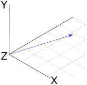
Fig 1: A visual representation of a three-dimensional vector.
Vectors will give our renderer the mathematical foundation for modeling rays of light. Our renderer will represent vectors in terms of their co-ordinates from the origin. For example, the two-dimensional vector \(V=(1,1)\) can be visualized as a line starting at the origin (0,0) and extending to the point (4,2).
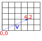
Fig 2: A visual representation of the vector (4,2).
To represent vectors in our Rust renderer, we will use two structs: Vector2d for the two-dimensional case, and Vector3d for the three-dimensional case. Because we may want to create vectors of both floating-point and integer types in our rendering application, it's useful to implement these as generic types, as follows:
#![allow(unused)]
fn main() {
pub struct Vector2d<T> {
    pub x: T,
    pub y: T
}
impl<T> Vector2d<T> {
    fn new(x: T, y: T) -> Self {
        Vector2d { x, y }
    }
}

pub struct Vector3d<T> {
   pub x: T,
   pub y: T,
   pub z: T
}
impl<T> Vector3d<T> {
    pub fn new(x: T, y: T, z: T) -> Self {
        Vector3d { x, y, z }
    }
}
}
For the remainder of these examples, I'll focus on the implementations for the Vector3d class, which are essentially the same as for Vector2d.
The components of vectors can be accessed as simple properties on the struct (vec.x, vec.y etc.). For some algorithms, it is also useful to be able to iterate over the components of vectors, so in addition to allowing access by property, we overload the index operator to allow vec[0], vec[1] etc. To overload operators in Rust, we import the relevant trait from std::ops and provide an impl statement, as below:
#![allow(unused)]
fn main() {
use std::ops::Index;

impl<T> Index<usize> for Vector3d<T> {
    type Output = T;
    fn index(&self, index: usize) -> &Self::Output {
        match index {
            0 => &self.x,
            1 => &self.y,
            2 => &self.z,
            _ => panic!("Index out of bounds")
        }
    }
}
}
Adding and subtracting vectors
To add two vectors we just add up the components item-by-by item. So if we have two three-dimensional vectors \(V\) and \(W\), their sum is a new vector where each component is the sum of the corresponding components of V and W:
\[ V=(1,3,5) \\ W=(2,4,6) \\ V+W=(Vx+Wx,Vy+Wy,Vz+Wz) \\ =(1+2,3+4,5+6) \\ =(3,7,11) \\ \]
The geometric interpretation of vector addition is equivalent to imagining the two vectors arranged to form a path, where the first vector starts at the origin, and the second vector starts where the first terminates. If we follow the second vector to its terminus, we find outselves at the co-ordinates representing the components of the new vector. The diagram below shows this for two vectors \(V=(4,2)\) and \(W=(−1,3)\), giving the expected result of \(V+W=(3,5)\)
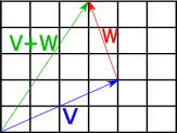
Fig 3: Geometric interpretation of vector addition.
As one might expect, subtraction is also applied elementwise:
\[ V=(1,3,5) \\ W=(2,4,6) \\ V−W=(V_x−W_x,V_y−W_y,V_z−W_z) \\ =(1−2,3−4,5−6) \\ =(−1,−2,−1) \\ \] The geometric interpretation of vector subtraction is equivalent to imagining both vectors as paths originating at the origin, and finding the vector which connects the second operand to the first operand. The diagram below shows this for two vectors \(V=(5,2)\) and \(W=(3,5)\). Subtracting V from W gives us \(W−V=(−2,3)\).
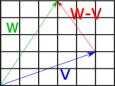
Fig 4: Geometric interpretation of vector subtraction.
To implement these operations in Rust, we import the std::ops::Add and std::ops::Sub traits and provide implementations with impl statements. Things get a little tricky here, because the implementations will need to use the + and - operator on the vector components; however, because we are using generics, we are unable to guarantee that the components (which could be of any type) actually support these operators. To get around this, we can use the num::Real trait as a trait bound on our implementations, meaning that the Vector structs can only be created with numeric types which represent real numbers.
#![allow(unused)]
fn main() {
use num::Real;

impl<T:Real> Vector3d<T> {
    fn new(x: T, y: T, z: T) -> Self {
        Vector3d { x, y, z }
    }
}
}
The impl<T:Real statement means that we are implementing the new constructor only for types which represent real numbers. With this in place, we can import the Add and Sub traits from the std::ops crate, and define our addition and subtraction operations:
#![allow(unused)]
fn main() {
use std::ops::{Index, Add, Sub};

impl <T:Real> Add for Vector3d<T> {
    type Output = Vector3d<T>;
    fn add(self, other: Self) -> Self::Output {
        Vector3d::new(self.x + other.x, self.y + other.y, self.z + other.z)
    }
}
impl <T:Real> Sub for Vector3d<T> {
    type Output = Vector3d<T>;
    fn sub(self, other: Self) -> Self::Output {
        Vector3d::new(self.x - other.x, self.y - other.y, self.z - other.z)
    }
}
}
Vector negation
Negating a vector can be achieved by negating each component. It results in a vector of the same magnitude pointing in the opposite direction. We can implement this in a similar manner to the other operations -- importing the Neg trait from std::ops and providing an implementation.
#![allow(unused)]
fn main() {
impl <T:Real> Neg for Vector3d<T> {
    type Output = Vector3d<T>;
    fn neg(self) -> Self::Output {
        Vector3d::new(-self.x, -self.y, -self.z)
    }
}
}
Scalar multiplication and division
A vector can be multiplied and divided by a scalar value. To implement this, we just apply the multiplication/division operation element-wise to the vector.
So scalar multiplication will look like this:
\[ V=(1,3,5) \\ n=10 \\ Vn=(V_x+n,V_y+n,V_z+n) \\ =(1x10,3x10,5x10) \\ =(10,30,50) \\ \] ...and scalar division will look like this:
\[ V=(1,3,5) \\ n=2 \\ Vn=(V_xn,V_yn,V_zn) \\ =(12,32,52) \\ =(0.5,1.5,2.5) \\ \]
The geometric interpretation of these operations that they scale the vector's magnitude by the scalar degree. So the vector \(V=(2,2)\) (of length two) multipled by 2 will become \((4,4)\), which is of length 4; dividing this by 2 returns the original value of \(V\)
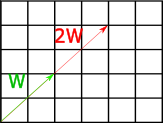
Fig 5: Geometric interpretation of multiplying a vector by a scalar.
In Rust code, this is pretty much the same as what we did for the Add and Sub operations -- we again import the relevant traits from the std::ops library, and provide implementations.
#![allow(unused)]
fn main() {
use std::ops::{Index, Add, Sub, Mul, Div};

impl <T:Real> Mul for Vector3d<T> {
    type Output = Vector3d<T>;
    fn mul(self, other: Self) -> Self::Output {
        Vector3d::new(self.x * other.x, self.y * other.y, self.z * other.z)
    }
}
impl <T:Real> Div for Vector3d<T> {
    type Output = Vector3d<T>;
    fn div(self, other: Self) -> Self::Output {
        Vector3d::new(self.x / other.x, self.y / other.y, self.z / other.z)
    }
}
}
The dot product of two vectors
The dot product gives us a measure of the similarity between two vectors. This will be useful for doing things like calculating the angle at which light strikes a surface. To take the dot product of two vectors, we multiply their components element-wise, and sum the result:
\[ V \cdot W = \sum_{i=1}^n V_iW_i\\ \]
For example, the dot product of \(V = (2, 3, 4\) and \(W = (4, 3, 2)\) is:
\[ (V_xW_x, V_yW_y, V_zW_z)\\ = (2 x 4, 3 x 3, 4 x 2)\\ = (8, 9, 8) \]
The dot product is useful because of its relationship to the angle between the two vectors -- it is equal to the product of the lengths of the vectors times the cosine of the angle between them:
\[ V \cdot W = |V| |W| cos \theta \]
A consequence of this is that if both vectors are normalized to have a length of one (see: 'Vector Normalization' below), the magnitudes can be disregarded by removing the first term from the above equation, so we have:
\[ \hat{V} \cdot \hat{W} = cos \theta \]
So the dot product allows us to directly calculate the cosine of the angle between two vectors. When the dot product is 0, this means that the two vectors are exactly perpendicular; when it is 1, it means that the two vectors are parallel, and when it is -1, the vectors point in the opposite directions.
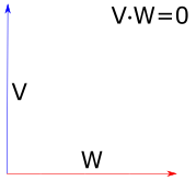
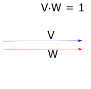
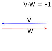
Fig 6: Geometric interpretation of the dot product for unit vectors.
To implement the dot product in our Rust renderer, we add a dot() method to the impl block for our Vector structs:
#![allow(unused)]
fn main() {
impl<T:Real Vector3d<T> {
    pub fn new(x: T, y: T, z: T) -> Self {
        Vector3d { x, y, z }
    }
    pub fn dot(&self, other: &Self) -> T {
        self.x * other.x + self.y * other.y + self.z * other.z
    }
}
}
The cross product of two vectors
The cross product of two three-dimensional vectors allows us to find a vector which is orthogonal to both of them. It can be calculated as follows:
\[ (V \times W)_x = V_yW_z - V_zW_y\\ (V \times W)_y = V_zW_x - V_xW_z\\ (V \times W)_z = V_xW_y - V_yW_x\\ \]
One way to remember this pattern is to observe that for each component of the output vector (x, y, z), the calculation uses the next two components in the sequence. So for \((V \times W)_x\), we use the y and z components of the two input vectors; \((V \times W)_y\) uses z and x, and \((V \times W)_z\) uses x and y. The calculation then proceeds as follows. For each output component:
- Identify the two target components for this output component. So for \((V \times W)_x\), we are dealing with y and z.
- Take the first component (from the target components) on the first input vector, and multiply it with the second component on the second input vector. Our target components are y and z, and our input vectors are \(V\) and \(W\) -- so we multiply \(V_y\) and \(W_z\)
- Take the second component (from the target components) on the first input vector, and multiply it with the first component on the second input vector. Our target components are y and z, and our input vectors are \(V\) and \(W\) -- so we multiply \(V_z\) and \(W_y\)
- Subtract the second multiplication result from the first.
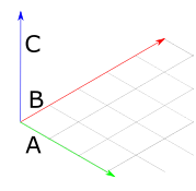
The geometric interpretation of the cross product is that, given two input vectors, it returns a third vector which is orthogonal to the two input vectors. In the image below, vectors \(A\) and \(B\) form a plane in the X-Z dimension, so their cross-product is a vector which points straight up along the Y axis. The angle between this vector and each of the others is 90 degrees.
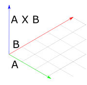
*Fig 7: Geometric interpretation of the cross product.
To implement the cross product for our Vector3d struct, we add it to the relevant impl block. Note that we don't need to do this for Vector2d, as the cross-product is not well-defined for 2d vectors.
#![allow(unused)]
fn main() {
impl<T:Real> Vector3d<T> {
    pub fn new(x: T, y: T, z: T) -> Self {
        Vector3d { x, y, z }
    }
    pub fn dot(&self, other: &Self) -> T {
        self.x * other.x + self.y * other.y + self.z * other.z
    }
    pub fn cross(&self, other: &Self) -> Self {
        Vector3d::new(self.y * other.z - self.z * other.y,
                      self.z * other.x - self.x * other.z,
                      self.x * other.y - self.y * other.x)
    }
}
}
To test this method, we can consider the case of our typical representation of a 3D space with axes, where each axis is a unit vector extending in one dimension only. So we have an X axis \((1, 0, 0)\), Y axis \((0, 1, 0)\), and Z axis \((0, 0, 1)\). We can retrieve the third axis given two others using the cross product:
#![allow(unused)]
fn main() {
#[test]
fn test_vector_3d_cross() {
    let v1 = Vector3d::new(1.0, 0.0, 0.0);
    let v2 = Vector3d::new(0.0, 1.0, 0.0);
    let v3 = Vector3d::new(0.0, 0.0, 1.0);
    assert_eq!(v1.cross(&v2), v3);
    assert_eq!(v3.cross(&v1), v2);
    assert_eq!(v2.cross(&v3), v1);
}
}
However, it should be noted that order matters when calculating the cross product. This because there are always two orthogonal vectors given two inputs -- one in each direction. So if we take the cross products in the above test and reverse the operands, we get the inverse result:
#![allow(unused)]
fn main() {
#[test]
fn test_vector_3d_cross_negative() {
    let v1 = Vector3d::new(1.0, 0.0, 0.0);
    let v2 = Vector3d::new(0.0, 1.0, 0.0);
    let v3 = Vector3d::new(0.0, 0.0, 1.0);
    assert_eq!(v2.cross(&v1), -v3);
    assert_eq!(v1.cross(&v3), -v2);
    assert_eq!(v3.cross(&v2), -v1);
}
}
Normalization
To normalize a vector we compute a new vector with the same direction but with length one. To achieve this, we first need a way to compute the length of a vector. This can be achieved by taking the square-root of the sum of squared components. So if \(V\) is a vector with \(n\) components, and lower-case \(v_n\) represents each component, the length is calculated as:
\[ |V| = \sqrt{v_1^2 + v_2^2 ... v_n^2 }\\ \]
To get the normalized vector, we divide it by the length, which is achieved by applying the division to each component:
\[ \hat{V} = \frac{V}{|V|}\\ = (\frac{V_x}{|V|}, \frac{V_y}{|V|}, \frac{V_z}{|V|})\\ \]
In our Rust code, we can achieve this with a few additional methods for our Vector implementations -- squared_length(), length() and normalized():
#![allow(unused)]
fn main() {
impl<T:Real> Vector3d<T> {
    ...
    pub fn squared_length(&self) -> T {
        self.x * self.x + self.y * self.y + self.z * self.z
    }
    pub fn length(&self) -> T {
        self.squared_length().sqrt()
    }
    pub fn normalized(&self) -> Self {
        Vector3d {
            x: self.x / self.length(),
            y: self.y / self.length(),
            z: self.z / self.length()
        }
    }
}
Miscellaneous Operations
There are several other methods included for Vectors in the C++ pbrt implementation. These include;
- Methods for retrieving the max and min component of a vector (
min_component()andmax_component()) - A method for retrieving the index of the component with the largest value (
max_dimension()) - Component-wise minimum and maximum operations (
min()andmax()) - A method for permuting a vector based on input indices (
permute())
Generating a coordinate system from an input vector
We will frequently want to construct a local coordinate system given only a single 3D vector.
Because the cross product of two vectors is orthogonal to both, we can apply the cross product two times to get a set of three orthogonal vectors for the coordinate system. The corresponding method on our Rust implemention of Vector3d looks like this:
#![allow(unused)]
fn main() {
impl<T:Real> Vector3d<T> {
    ...
    pub fn coordinate_system(&self) -> (Self, Self) {
        let y = if self.x.abs() > self.y.abs() {
            Vector3d::new(-self.z, zero(), self.x) /
            (self.x * self.x + self.z * self.z).sqrt()
        } else {
            Vector3d::new(zero(), self.z, -self.y) /
            (self.y * self.y + self.z * self.z).sqrt()
        };
        (self.cross(&y), y)
    }
}
}
One thing of note here is the zero() function imported from num -- this allows us to provide a 0 value as default without specifying a type. If we used 0.0 here, the Rust compiler would complain, as this would commit us to a vector of floats, but we have defined Vector as a generic type.
In a similar manner to the tests for the cross product, we can test this method by passing it a unit vector in X (\(1, 0, 0)\) -- we expect it to return corresponding orthogonal vectors in Y and Z. We can further convince ourselves that these are orthogonal using the dot product, as we expect a value of zero for the dot product of two orthogonal vectors.
#![allow(unused)]
fn main() {
#[test]
fn test_vector_3d_coordinate_system() {
    let v = Vector3d::new(1.0, 0.0, 0.0).normalized();
    let (v1, v2) = v.coordinate_system();
    assert_eq!(v1, Vector3d::new(0.0, -1.0, 0.0));
    assert_eq!(v2, Vector3d::new(0.0, 0.0, 1.0));
    assert_eq!(v1.dot(&v2), 0.0);
    assert_eq!(v2.dot(&v1), 0.0);
    assert_eq!(v.dot(&v1), 0.0);
    assert_eq!(v.dot(&v2), 0.0);
}
}
Geometry and Transformations
1.2 Points
A point is a location in 2d or 3d space. We can represent points in terms of their co-ordinates -- so \(x,y\) for 2d and \(x,y,z\) for 3d points. Although this is the same basic representation as vectors, the fact that they represent positions instead of directions means that they will be treated differently. The Rust structs for points look similar to vectors:
#![allow(unused)]
fn main() {
pub struct Point2D<T> {
    pub x: T,
    pub y: T,
}
impl<T: Scalar> Point2D<T> {
    pub fn new(x: T, y: T) -> Self {
        Point2D{x, y}
    }
}
pub struct Point3D<T> {
    pub x: T,
    pub y: T,
    pub z: T,
}
impl<T: Scalar> Point3D<T> {
    pub fn new(x: T, y: T, z: T) -> Self {
        Point3D{x, y, z}
    }
}
}
The C++ pbrt implementation also includes methods for:
- Converting a 3d point to 2d by dropping the 'z' component.
- Converting points of one type (e.g. floats) to another (e.g. int)
- Converting a point of one type to a vector of another type.
To achieve this in Rust, we can add appropriate methods to the Point implementations.
To do the type conversions, we need to add additional type parameters. Taking the conversion of Point3d betweent types as an example:
#![allow(unused)]
fn main() {
impl<T: Scalar> Point3d<T> {
    ...
    pub fn from<U, V: From<U>>(p: Point3d<U>) -> Point3d<V> {
        Point3d{x: p.x.into(), y: p.y.into(), z: p.z.into()}
    }
}
}
The from<U, V> statement declares two generic types, then (p: Point3d<U>) -> Point3d<V> specifies that we will take an argument of one type and convert to the other. The trait bound on V, V: From<U> means that we will only support types which support this conversion. Types that satisfy this trait will have an into() method which will do the cast for us.
Operations on vectors and points
We can add or subtract vectors and points by applying the addition/subtraction operation componentwise. Adding and subtracting vectors and points has the affect of offsetting the point along the vector. So if we think of a vector as a path, if we start at point A and add the vector, we end up at point B. Subtraction has the opposite affect -- if we start at point A and subtract the vector, we walk in the opposite direction of its trajectory.
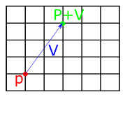
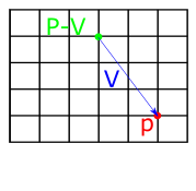
Fig 1: Geometrical interpretation of vector-point addition (left) and vector-point subtraction (right).
To implement these in Rust, we can follow the same pattern as for vectors -- importing the std::ops::Add and std::ops::Sub traits and providing implementations.
#![allow(unused)]
fn main() {
impl<T: Scalar> Add<Vector3d<T>> for Point3d<T> {
    type Output = Self;
    fn add(self, other: Vector3d<T>) -> Self {
        Point3d{x: self.x + other.x, y: self.y + other.y, z: self.z + other.z}
    }
}
impl<T: Scalar> Sub<Vector3d<T>> for Point3d<T> {
    type Output = Self;
    fn sub(self, other: Vector3d<T>) -> Self {
        Point3d{x: self.x - other.x, y: self.y - other.y, z: self.z - other.z}
    }
}
}
Subtracting two points gives us the vector between them, as shown below:
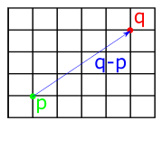
This means that we can easily find the distance between two points by subtracting them and taking the length of the resulting vector. We can implement this by using the length() method added to the Vector structs in the previous chapter. First we implement Sub for points, which returns a vector:
#![allow(unused)]
fn main() {
impl<T: Scalar> Sub<Point3d<T>> for Point3d<T> {
    type Output = Vector3d<T>;
    fn sub(self, other: Self) -> Self::Output {
        Vector3d{x: self.x - other.x, y: self.y - other.y, z: self.z - other.z}
    }
}
}
Then we add the distance method to the impl block for the Point structs. I've also added distance_squared following the c++ pbrt implementation:
#![allow(unused)]
fn main() {
impl<T: Scalar> Point3d<T> {
    ...
    pub fn distance(self, other: Self) -> T {
        return (self - other).length();
    }
    pub fn distance_squared(self, other: Self) -> T {
        return (self - other).squared_length();
    }
}
}
Following the pbrt book, we also include methods for adding points and scalar multiplication with a point, which are similar to the implementation for Vector.
Linear interpolation
It's often necessary to interpolate between two points. For example, given the two points \((x_0, y_0)\) and \((x_1, y_1)\) in the image below, we may want to find some intermediate point \((x, y)\).
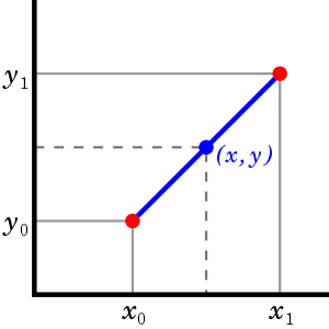
Fig 2: Linear interpolation
The goal of interpolation is to be able to return arbitrary points which lie between two values. So we are aiming for a method with the following signature:
#![allow(unused)]
fn main() {
impl<T: Scalar> Point2d<T> {
    ...
    pub fn lerp(&self, t: T, p0: Point2d<T>, p1: Point2d<T>) -> Point2d<T>;
}
}
We want this method to return a point at p0 when the t argument is 0, and a point at p1 when the value of t is 1. We can interpolate between two points by imagining a straight line between them, as in the above diagram, then picking points along it. We can get a line like this by finding the vector between the two points (using subtraction, as implemented earlier), then multiplying the resulting vector by some amount. For example, if we scale it by 0.5, we get a vector pointing in the same direction, but with half the length. We then just need to add the starting point (if we just took the x and y values of the vector, our line would start from the origin).
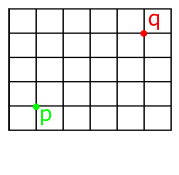
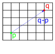
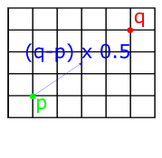
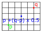
Fig 3: Linear interpolation by finding the vector between two points then scaling it.
The above process can be translated into code as follows:
#![allow(unused)]
fn main() {
impl<T: Scalar> Point2d<T> {
    ...
        pub fn lerp(self, other: Self, t: T) -> Self {
        return self + (other - self) * t;
    }
}
}
Miscellaneous point operations
The c++ implementation of pbrt includes:
- operations for returning component-wise min and max
- operations for applying floor(), ceil(), and abs() to each component and returning a new point
- a permute operation which returns a new point with components permuted based on some indices
These are mostly straightfoward, although it should be noted that floor() and ceil() are only defined for floating-point types, so we need to define these in a separate impl block which specifies the Float trait bound:
#![allow(unused)]
fn main() {
impl<T: Scalar + Float> Point3d<T> {
    pub fn floor(self) -> Self {
        Point3d::new(self.x.floor(), self.y.floor(), self.z.floor())
    }
    pub fn ceil(self) -> Self {
        Point3d::new(self.x.ceil(), self.y.ceil(), self.z.ceil())
    }
}
}
Geometry and Transformations
1.3 Normals
A normal vector is a vector which is perpendicular to a surface at particular point. To calculate it, we take the cross product of any two nonparallel vectors which are tangent to the surface at a point.
For example, in the diagram below, C is a normal vector of the plane formed by A and B:
Normals look a lot like vectors, but behave differently, particularly when it comes to transformations. My Rust implementation of pbrt will follow the original implementation in defining them as a separate type, Normal3d.
Normal3d includes all of the functionality of Vector3d, with the exception of the cross product.
The c++ pbrt implementation also includes a method called FaceForward, which flips a surface normal so that it lies in the same hemisphere as a given vector. This is implemented for all four combinations of Normals and Vectors, and provides an opportunity to further experiment with Rust generics. Here's the FaceForward trait:
#![allow(unused)]
fn main() {
/// Flip a surface normal so that it lies in the same hemisphere as a given vector.
/// This is useful for computing the reflection direction.
/// This trait provides default behavior for any combination of vector types.
pub trait FaceForward<T: Dot<T, U> + Clone + Neg<Output = T>, U: Scalar>: Dot<T, U> {
    fn face_forward(&self, other: T) -> T {
        if self.dot(&other) < zero() {
            other.clone()
        } else {
            -other.clone()
        }
    }
}
/// Implements the FaceForward trait for any combination of vector types.
impl<U: Scalar, T: Dot<T, U> + Clone + Neg<Output = T>, V: Dot<T, U>> FaceForward<T, U> for V{}
}
This trait provides default behaviour for any type which can perform a dot() operation with some other type, where that type can be cloned and negated.
Geometry and Transformations
1.4 Rays
A ray is a semi-infinite line specified by a point \(o\) representing its origin and a vector \(d\) representing its direction.

The parametric form of a ray expresses it as a function of a scalar value \(t\), giving the set of points that the ray passes through:
\[ r(t) = o + td \quad 0 \le t < \infty \]
The Ray class implements an at(t) method, allowing a caller to retrieve a point along the ray:
#![allow(unused)]

fn main() {
pub struct Ray<T> {
    pub origin: Point3d<T>,
    pub direction: Vector3d<T>,
    pub t_max: Cell<T>,
    pub time: T
}
impl<T: Scalar> Ray<T> {
    pub fn new(origin: Point3d<T>, direction: Vector3d<T>, tmax: T, time: T) -> Self {
        Ray {
            origin,
            direction,
            t_max: Cell::new(tmax),
            time
        }
    }
    pub fn default() -> Self {
        Ray {
            origin: Point3d::<T>::new(T::zero(), T::zero(), T::zero()),
            direction: Vector3d::<T>::new(T::zero(), T::zero(), T::zero()),
            t_max: Cell::new(T::inf()),
            time: T::zero()
        }
    }
    pub fn at(&self, t: T) -> Point3d<T> {
        self.origin + self.direction * t
    }
}
}
As with the c++ implementation, the Ray struct provides an all-argument constructor as well as a default() which sets the origin, direction and time values to 0, and t_max to infinity. The Ray also includes a member variable that limits the ray to a segment along its infinite extent. This field, tMax, allows us to restrict the ray to a segment of points. Following the c++ pbrt implementation, this fields needs to be mutable to allow a caller to modify it (this will be useful when recording the points where the ray intersects with an object). In order to make a single field mutable in rust, we need to use the Cell<T> struct. This will allow a caller to set and get the value using the set and get methods on Cell<T>.
1.4.2 Ray Differentials
The c++ pbrt implementation includes a subclass of Ray with additional information about two auxiliary rays. These extra rays represent camera rays offset by one sample in the \(x\) and \(y\) direction from the main ray on the film plane. By moving the Ray methods out to a trait and implementing them for both Ray and RayDifferential, we can enable geometry methods which act on both Rays and RayDifferentials without caring which underlying type they are dealing with. Here's what the RayMethods trait looks like:
#![allow(unused)]
fn main() {
trait RayMethods<T> {
    fn origin(&self) -> Point3d<T>;
    fn direction(&self) -> Vector3d<T>;
    fn at(&self, t: T) -> Point3d<T>;
    fn t_max(&self) -> &Cell<T>;
    fn time(&self) -> T;
}
}
We can then add impl blocks returning the appropriate fields for both Ray and RayDifferential. RayDifferential has a few extra fields and methods:
#![allow(unused)]
fn main() {
pub struct RayDifferential<T> {
    pub origin: Point3d<T>,
    pub direction: Vector3d<T>,
    pub t_max: Cell<T>,
    pub time: T,
    pub rx_origin: Point3d<T>,
    pub ry_origin: Point3d<T>,
    pub rx_direction: Vector3d<T>,
    pub ry_direction: Vector3d<T>,
    pub has_differentials: bool
}
impl<T: Scalar> RayDifferential<T> {
    pub fn new(origin: Point3d<T>, direction: Vector3d<T>, tmax: T, time: T) -> Self {
        RayDifferential {
            origin: origin,
            direction: direction,
            rx_origin: Point3d::<T>::new(T::zero(), T::zero(), T::zero()),
            rx_direction: Vector3d::<T>::new(T::zero(), T::zero(), T::zero()),
            ry_origin: Point3d::<T>::new(T::zero(), T::zero(), T::zero()),
            ry_direction: Vector3d::<T>::new(T::zero(), T::zero(), T::zero()),
            t_max: Cell::new(tmax),
            time: time,
            has_differentials: false
        }
    }
    pub fn default() -> Self {
        RayDifferential {
            origin: Point3d::<T>::new(T::zero(), T::zero(), T::zero()),
            direction: Vector3d::<T>::new(T::zero(), T::zero(), T::zero()),
            rx_origin: Point3d::<T>::new(T::zero(), T::zero(), T::zero()),
            rx_direction: Vector3d::<T>::new(T::zero(), T::zero(), T::zero()),
            ry_origin: Point3d::<T>::new(T::zero(), T::zero(), T::zero()),
            ry_direction: Vector3d::<T>::new(T::zero(), T::zero(), T::zero()),
            t_max: Cell::new(T::inf()),
            time: T::zero(),
            has_differentials: false
        }
    }
    pub fn from_ray(ray: &Ray<T>) -> Self {
        RayDifferential::new(ray.origin, ray.direction, ray.t_max.get(), ray.time)
    }
    pub fn scale_differentials(&mut self, s: T) {
        self.rx_origin = self.origin + (self.rx_origin - self.origin) * s;
        self.ry_origin = self.origin + (self.ry_origin - self.origin) * s;
        self.rx_direction = self.direction + (self.rx_direction - self.direction) * s;
        self.ry_direction = self.direction + (self.ry_direction - self.direction) * s;
    }
}
}
The RayDifferential the rx_ fields describe origin and direction information about these rays, and the 'ScaleDifferentials' method updates the differential rays for an estimated sample spacing of s. Finally, a from_ray_ constructor allows us to create a RayDifferential from a Ray.
Geometry and Transformations
1.5 Bounding Boxes
A bounding box describes the extent of some region of space. Bounding boxes will be useful for our renderer, because if we divide a space into bounding boxes we can make early decisions about whether calculations need to be done in a particular area (so if you imagine we have 10 complex objects in a box, we can first check if a calculation need sto be done for the box at all, and avoid it if not).
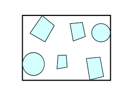
Fig 1.1: A bounding box around a set of objects in two dimensions
We can represent a bounding box in terms of it's min and max bounds, which are points in space. Here are what the structs look like:
#![allow(unused)]
fn main() {
pub struct Bounds2d<T> {
    pub min: Point2d<T>,
    pub max: Point2d<T>,
}
pub struct Bounds3d<T> {
    pub min: Point3d<T>,
    pub max: Point3d<T>,
}
}
The impl blocks for the Bounds structs provide a constructor which automatically selects the min and max points from the two arguments, as well as a default method that setting the extent to an invalid configuration, which violates the invariant that pMin.x <= pMax.x. This allows operations involving empty boxes e.g., Union() to return the correct result (otherwise they would contain everything and always be true). I've also included a new_from_point method for returning a box from a single point.
#![allow(unused)]
fn main() {
impl<T: Scalar> Bounds3d<T> {
    pub fn new(p1: Point3d<T>, p2: Point3d<T>) -> Self {
        let min = Point3d::<T>::new(
            p1.x.min(p2.x),
            p1.y.min(p2.y),
            p1.z.min(p2.z)
        );
        let max = Point3d::<T>::new(
            p1.x.max(p2.x),
            p1.y.max(p2.y),
            p1.z.max(p2.z)
        );
        Bounds3d {
            min,
            max
        }
    }
    pub fn new_from_point(p: Point3d<T>) -> Self {
        Bounds3d {
            min: p,
            max: p
        }
    }
    pub fn default() -> Self {
        Bounds3d {
            min: Point3d{x: T::inf(), y: T::inf(), z: T::inf()},
            max: Point3d{x: -T::inf(), y: -T::inf(), z: -T::inf()}
        }
    }
}
}
The c++ pbrt implementation also has an overloaded 'Union' method for adding both points and other boxes to boxes. We can achieve this in rust with traits as follows:
#![allow(unused)]
fn main() {
trait Union<T> {
    fn union(&self, other: &T) -> Self;
}
impl<T: Scalar> Union<Point2d<T>> for Bounds2d<T> {
    fn union(&self, other: &Point2d<T>) -> Self {
        Bounds2d {
            min: Point2d {
                x: self.min.x.min(other.x),
                y: self.min.y.min(other.y)
            },
            max: Point2d {
                x: self.max.x.max(other.x),
                y: self.max.y.max(other.y)
            }
        }
    }
}
impl<T: Scalar> Union<Bounds2d<T>> for Bounds2d<T> {
    fn union(&self, other: &Bounds2d<T>) -> Self {
        Bounds2d {
            min: Point2d {
                x: self.min.x.min(other.min.x),
                y: self.min.y.min(other.min.y)
            },
            max: Point2d {
                x: self.max.x.max(other.max.x),
                y: self.max.y.max(other.max.y)
            }
        }
    }
}
}
This lets us call union() with either a Point or another Bounds, and have the compiler choose the correct method.
Geometry and Transformations
1.6 Transformations
A transformation is a mapping from points to points or from vectors to vectors. In 3D graphics, we are most interested in translations (moving from position to position), scaling, and rotation around an axis.
It turns out that we can express these translations in 4x4 matrices, which, when multiplied with a vector or point, will result a new vector/point with the translation applied. The same set of matrices will work for both vectors and points To do this, we first convert our representation of vectors and points into a single, 4 element representation: their homogeneous coordinates. The additional component will be zero for a vector, and a non-zero value for points. So both points and vectors will look like this:
\[ p = (x, y, z, 1) \\ v = (x, y, z, 0) \]
This representation is very convenient, because it means that the operations we might perform on points and vectors will reflect their geometric interpretation. For example, if we subtract two points, we get a vector:
\[ (8, 4, 2. 1) - (3, 2, 1, 1) = (5, 2, 1, 0) \]
And adding two vectors gives us another vector:
\[ (0, 0, 1, 0) - (1, 0, 0, 0) = (1, 0, 1, 0) \]
Once we have 4-element tuples like those above, we can construct 4x4 matrices which, when multipled with a point or vector, result in the desired transformation.
Scaling
If we want to scale each element of a point or vector, we can construct a matrix like this:
\[ \begin{bmatrix} 5 & 0 & 0 & 0\\ 0 & 5 & 0 & 0\\ 0 & 0 & 5 & 0\\ 0 & 0 & 0 & 1 \end{bmatrix} \]
Multiplying this with a vector or point will result in the \(x, y, z\) values of the point being multiplied by 5, with the \(w\) value preserved (so scaling a point returns a point, and scaling a vector returns a vector). This is shown below. To multiply a 4-vector and a matrix, we take its dot product with each row in the matrix.
\[ \begin{bmatrix} 5 & 5 & 5 & 1 \end{bmatrix} \begin{bmatrix} 5 & 0 & 0 & 0\\ 0 & 5 & 0 & 0\\ 0 & 0 & 5 & 0\\ 0 & 0 & 0 & 1 \end{bmatrix}= \begin{bmatrix} 25 & 25 & 25 & 1 \end{bmatrix} \]
Translation
For translation, we just want to add some scalar value to each element. To do that, we can construct a matrix like this one:
\[ \begin{bmatrix} 1 & 0 & 0 & T_x\\ 0 & 1 & 0 & T_y\\ 0 & 0 & 1 & T_z\\ 0 & 0 & 0 & 1 \end{bmatrix} \]
To understand this, we can imagine a point \((3, 3, 3, 1\)) which we want to translate by \(1, 0, 0\). We can just focus on the \(x\) axis as this is the only one we expect to change. We take our input vector and take its dot product with the row vector \((1, 0, 0, 1\)):
\[ (3, 3, 3, 1) \cdot (1, 0, 0, 1)\\ = 3 \times 1 + 3 \times 0 + 3 \times 0 + 1 \times 1 \\ = 3 + 1 \]
So -- the '1' in the first entry of row 1 means we start with the original value of x, then all others are set to zero except for the final value, which will get multipied by 1. To take the dot product, we sum those values, which gives us the expected result of 3 + 1 for x. The translation happens because we multiply the final value of the row by the point's \(w\) value of 1. This has the consequence that translation has no impact on a vector, which makes sense, as vectors have no position.
Rotation
To understand how to construct rotation matrices, it's useful to first understand the notion of basis vectors. The basis vectors are a set of unit vectors which lie along the axes of a co-ordinate system.
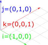
Figure 1: The basis vectors \(\hat{i}\), \(\hat{j}\) and \(\hat{k}\), which are unit vectors parallel to the \(x\), \(y\) and \(z\) axes.
\(\hat{i}\) typically describes the unit vector in \(x\); \(\hat{j}\) typically describes the unit vector in \(y\); and \(\hat{k}\) typically describes the unit vector in \(z\). So the basis vectors are:
\[ \hat{i} = \begin{bmatrix} 1 \\ 0 \\ 0 \\ \end{bmatrix} \quad \hat{j} = \begin{bmatrix} 0 \\ 1 \\ 0 \\ \end{bmatrix} \quad \hat{k} = \begin{bmatrix} 0 \\ 0 \\ 1 \\ \end{bmatrix} \]
We can think of all vectors in a given co-ordinate system as being composed of these basis vectors. For example, if we imagine this vector:
\[ v = \begin{bmatrix} 2 \\ 3 \\ 4 \end{bmatrix} \]
We can also imagine this as being composed of the basis vectors:
\[ v = 2\hat{i} + 3\hat{j} + 4 \hat{k} = 2 \begin{bmatrix} 1 \\ 0 \\ 0 \end{bmatrix} + 3 \begin{bmatrix} 0 \\ 1 \\ 0 \end{bmatrix} + 4 \begin{bmatrix} 0 \\ 0 \\ 1 \end{bmatrix} = \begin{bmatrix} 2 \\ 3 \\ 4 \end{bmatrix} \]
This means that if we can figure out how to transform the basis vectors, we can transform anything in their space. Let's think about how we might rotate the 2d basis vectors. Figure 2 shows our goal -- we want to take the vectors \(\hat{i}\) (in red) and \(\hat{j}\) (blue) and rotate them by the angle \(\theta\).
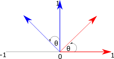
Figure 2: Rotating a vector in two dimensions.
To do this, we can imagine the two right-angled triangles formed by each basis vector and the target (rotated) vectors:
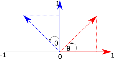
Figure 3: Using triangles to calculate the x and y values of rotated basis vectors.
To find the \(x\) and \(y\) components of the new vectors, we just need to find the length of the base (adjacent side) and height (opposite side) of each of these triangles.
The formulas for sine and cosine allow us to retrieve these values for the angle \(\theta\):
\[ cos(\theta) = \frac{adjacent}{hypotenuse}\\ sin(\theta) = \frac{opposite}{hypotenuse} \]
Because we are dealing with the basis vectors, which have a length of one, we can remove the division term, giving us:
\[ cos(\theta) = adjacent\\ sin(\theta) = opposite \]
So for the red basis vector (\(\hat{i}\)), the rotated version is given by:
\[ i_x = cos(\theta)\\ i_y = sin(\theta)\\ \]
For the blue basis vector, the same pattern applies, but because the base of the triangle is along the y-axis, the values correspond to different sides of the triangle: we get \(j_x\) from the length of the opposite side, and \(j_y\) from the length of the adjacent side. We also need to negate the x component, as it extends to the left of the x-axis:
\[ j_x = -sin(\theta)\\ j_y = cos(\theta)\\ \]
Now we know how to calculate the new x and y values for the basis vectors, we can construct a 2x2 matrix to transform them by a given angle:
\[ \begin{bmatrix} \cos \theta & -\sin \theta \\ \cos \theta & \sin \theta \\ \end{bmatrix} \]
To verify that this matrix works, we can multiply it with the basis vectors \(\hat{i} = (1, 0)\) and \(\hat{j} = (0, 1)\) used in the previous examples:
\[ R(\hat{i}) = \\ \begin{bmatrix} \cos \theta & -\sin \theta \\ \cos \theta & \sin \theta \\ \end{bmatrix} \begin{bmatrix} 1 \\ 0 \end{bmatrix}\\ = \begin{bmatrix} (1 \times \cos \theta) - (0 \times \sin \theta) \\ (1 \times \sin \theta) + (0 \times \cos \theta) \end{bmatrix}\\ = \begin{bmatrix} \cos \theta\\ \sin \theta\\ \end{bmatrix} \]
\[ R(\hat{j}) = \\ \begin{bmatrix} \cos \theta & -\sin \theta \\ \cos \theta & \sin \theta \\ \end{bmatrix} \begin{bmatrix} 0 \\ 1 \end{bmatrix}\\ = \begin{bmatrix} (0 \times \cos \theta) - (1 \times \sin \theta) \\ (0 \times \sin \theta) + (1 \times \cos \theta) \end{bmatrix}\\ = \begin{bmatrix} - \sin \theta\\ \cos \theta\\ \end{bmatrix} \]
To take this into three dimensions, we just need to add an extra dimension, and make it so that one dimension remains unchanged while we rotate the vector around the target axis. So we are looking for three matrices, one per rotation axis, which will leave that component of the vector unchanged whilst modifying the others to reflect the rotation.
\[ M_x = \begin{bmatrix} ? & ? & ? \\ ? & ? & ? \\ ? & ? & ? \\ \end{bmatrix} \quad M_y = \begin{bmatrix} ? & ? & ? \\ ? & ? & ? \\ ? & ? & ? \\ \end{bmatrix} \quad M_z = \begin{bmatrix} ? & ? & ? \\ ? & ? & ? \\ ? & ? & ? \\ \end{bmatrix} \]
It's useful to start with the z-axis, because we've actually already covered the meat of it! A 2d rotation can also be imagined as a 3d rotation around the z-axis -- nothing moves in z, and we modify x and y to reflect the rotation. So all we need to do is take the 2d matrix used in the 2d example, move it into 3 dimensions, then ensure that the z axis stays constant. To fix the z axis, we can set the third column of the matrix to the basis vector \(\hat{k}\) = (\(0, 0, 1)\), and set the \(z\) value of the first and second columns (which represent the \(\hat{i}\) and \(\hat{j}\) basis vectors) to 0.
\[ M_z = \begin{bmatrix} \cos \theta & -\sin \theta & 0 \\ \sin \theta & \cos \theta & 0 \\ 0 & 0 & 1 \\ \end{bmatrix} \]
To derive the remaining matrices, we can go back to our original interpretation of rotation as finding the sides of triangles. However, this time we will fix x (which we can imagine projects out of the screen toward us), and manipulate the y and z axes.
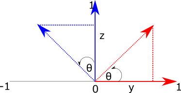
Figure 4: Rotating a vector around the \(x\) axis. We imagine \(x\) as extending out of the screen, and set the remaning axes to y (horizontal) and z (vertical).
The red triangle now represents the calculation for basis vector \(\hat{j}\), and the blue triangle now represents the calculation for \(\hat{k}\). To find the y-component of the transformed vector \(j_y\), we need the length of the base of the red triangle, which is \(\cos (\theta)\). To find \(j_z\), we need the length of the opposite side of the blue triangle, which is \(\sin (\theta)\).
For \(k\), we get the y-component from the inverse of the length of the opposite side of the blue triangle, so \(-\sin \theta\). The z-component comes from the length of the base of the blue triangle, which is \(\cos \theta\). So we have the following:
\[ j_y = \cos(\theta)\\ j_z = \sin(\theta)\\ k_y = -\sin(\theta)\\ k_z = \cos(\theta) \]
To create a matrix from these, we first want to ensure that the \(\hat{i}\) basis vector remains constant. To do this, we set the first column to that basis vector:
\[ M_x = \begin{bmatrix} 1 & ? & ? \\ 0 & ? & ? \\ 0 & ? & ? \\ \end{bmatrix} \]
We also want to ensure that the x-components of the y and z vectors are unaffected by the rotation, so we put zeros in their x-components:
\[ M_x = \begin{bmatrix} 1 & 0 & 0 \\ 0 & ? & ? \\ 0 & ? & ? \\ \end{bmatrix} \]
The middle column of this matrix represents \(\hat{j}\), and the third column represents \(\hat{k}\):
\[ M_x = \begin{bmatrix} 1 & 0 & 0 \\ 0 & \hat{j}_y & \hat{k}_y \\ 0 & \hat{j}_z & \hat{k}_z \\ \end{bmatrix} \]
So we can fill in the values we determined above using the triangle method:
\[ M_x = \begin{bmatrix} 1 & 0 & 0 \\ 0 & \cos(\theta) & -\sin(\theta) \\ 0 & \sin(\theta) & \cos(\theta) \\ \end{bmatrix} \]
To rotate around the Y-axis, we can just do the same trick again: take the triangle analogy above, then imagine that the Y axis is extending out from the screen, with X mapped to the vertical axis and Z mapped to the horizontal axis. We then get:
\[ k_x = \sin(\theta)\\ k_z = \cos(\theta)\\ i_x = \cos(\theta)\\ i_z = -\sin(\theta) \]
Once again, we want to ensure the rotation axis stays constant, so the middle column of our matrix needs to be set to \(\hat{j}\):
\[ M_x = \begin{bmatrix} ? & 0 & ? \\ ? & 1 & ? \\ ? & 0 & ? \\ \end{bmatrix} \]
We then set the \(y\) value of the other basis vectors to zero:
\[ M_x = \begin{bmatrix} ? & 0 & ? \\ 0 & 1 & 0 \\ ? & 0 & ? \\ \end{bmatrix} \]
The first column of this matrix represents \(\hat{i}\), and the final column represets \(\hat{k}\).
\[ M_x = \begin{bmatrix} i_x & 0 & k_x \\ 0 & 1 & 0 \\ i_z & 0 & k_z \\ \end{bmatrix} \]
So we can fill in the values from the triangle method:
\[ M_x = \begin{bmatrix} \cos(\theta) & 0 & \sin(\theta) \\ 0 & 1 & 0 \\ -\sin(\theta) & 0 & \cos(\theta) \\ \end{bmatrix} \]
Finally, to make these transformations compatible with the 4x4 transforms introduced earlier in the section, we need to add padding. This padding will be all zeros, except for the bottom right-hand element of the matrix, which ensures that the w-component of the input is preserved, so a rotated vector is a vector, and a rotated point is a new point. This gives us the following matrices:
\[ R_x(\theta) = \begin{bmatrix} 1 & 0 & 0 & 0\\ 0 & cos \theta & - sin \theta & 0\\ 0 & -sin \theta & cos \theta & 0\\ 0 & 0 & 0 & 1 \end{bmatrix} \]
\[ R_y(\theta) = \begin{bmatrix} cos \theta & 0 &- sin \theta & 0\\ 0 & 1 & 0 & 0\\ sin \theta & 0 & cos \theta & 0\\ 0 & 0 & 0 & 1 \end{bmatrix} \]
\[ R_z(\theta) = \begin{bmatrix} cos \theta & - sin \theta & 0 & 0\\ sin \theta & cos \theta & 0 & 0\\ 0 & 0 & 1 & 0\\ 0 & 0 & 0 & 1 \end{bmatrix} \]
Rotating around an arbitrary axis
So far we have covered the rotation matrices for the \(x\), \(y\) and \(z\) axes. What if we want to rotate around an arbitrary vector?

Figure 5: Rotating a vector around an arbitrary axis
Figure 5 visualizes the the problem -- we want to take the unit vector \(v\) and move it around the axis \(a\) by \(\theta^{\circ}\).
To simplify this problem, we can imagine \(v\) as being composed of two vectors: \(v_{\parallel}\), which is parallel to \(a\), and \(v_{\bot}\), which is perpendicular to \(a\). This is shown in Figure 6.

Figure 6: The vector \(v\) can be decomposed into \(v_{\parallel}\), which is parallel to \(a\), and \(v_{\bot}\), which is perpendicular to \(a\).
We can find \(v_{\parallel}\) by projecting \(v\) on to \(a\). The standard formula for a projection is:
\[ \frac{a \cdot b}{|a|^2}a \]
Because \(a\) is a unit vector, this simplifies to:
\[ v_{\parallel} = (v \cdot a)a \]
\(v_{\bot}\) can then be found by subtracting \(v_{\parallel}\) from \(v\):
\[ v_{\bot} = v - (v \cdot a) a \]
Because \(v = v_{\bot} + v_{\parallel}\), to get the rotated vector \(v'\), we can find the sum of the rotation of \(v_{\parallel}\) and \(v_{\bot}\). We already know that the rotation of \(v_{\parallel}\) will be \(v_{\parallel}\), because it is parallel to the axis of rotation \(a\). To find \(v_{\bot}\), we can re-orient our view such that we are looking straight down \(a\). This reduces the problem to a rotation in 2D:

Figure 7: The rotation of \(v_{\bot}\) can be viewed as a rotation in 2d
The base of this triangle gives us the x-component of \(v_{\bot}\), and the opposite side gives us the y-component. The base is equal to \(\cos \theta\), and the opposite is equal to \(\sin \theta\). We will need to multiply these by some new basis vectors in order to translate them into our initial frame. The horizontal axis in Figure 7 is easy to find: it's \(v_{\bot}\). If we imagine the view rotated slightly such that we can see \(a\) (Figure 8), it becomes clear that the vertical axis is one perpendicular to both \(v_{\parallel}\) and \(a\), which means we can obtain it from their cross product \(v_{\parallel} \times a\).

Figure 8: The vertical axis when rotating \(v_{\bot}\) is the cross-product of \(v_{\bot}\) and \(a\)
Summarizing the derivation, we can decompose \(v\) into \(v_{\parallel}\) and \(v_{\bot}\) as follows:
\[ v_{\parallel} = (v \cdot a)a \\ v_{\bot} = v - (v \cdot a) a \]
This allows us to express the rotation as:
\[ R(v) = R(v_{\parallel}) + R(v_{\bot}) \\ \]
No rotation is required for \(v_{\parallel}\) because it is parallel to the axis of rotation. The calculation of \(R(v_{\bot})\) can be thought of as a two-dimensional rotation, with each component multipled by a new basis vector to orient the circle of rotation correctly. The horizontal basis is \(v_{\bot}\), and the vertical basis is \(v_{\parallel} \times a\). This gives us:
\[ R(v) = v_{\parallel} + v_{\bot}\cos \theta + (v_{\parallel} \times a) \sin \theta \]
The Look-At Transformation
Given a point representing the location of a camera, a point the camera is looking at, and an 'up' vector which orients the camera along the vector described by the first two parameters, the look-at transformation maps from a left-handed co-ordinate system to one with the camera at the origin, looking along the z-axis, with the y-axis pointing upward. In other words, it lets us describe a camera position and orientation in "world-space" and provides a means of mapping between that space and the camera's viewpoint. The look-at transformation tells us what things look like from the camera's perspective.
To construct this transformation, we can use the same principles applied for the other transformations -- we create a matrix where each column describes the effect of the transformation on the basis vectors of a co-ordinate system.
The fourth column of the matrix gives the origin, and since our camera will be at the origin, we set this to the position of the camera in world space.
\[ position = (x, y, z, 1)\\ lookAt = (x, y, z, 1)\\ up = (x, y, z, 0)\\ \begin{bmatrix} ? & ? & ? & position_x\\ ? & ? & ? & position_y\\ ? & ? & ? & position_z\\ ? & ? & ? & 1\\ \end{bmatrix} \]
To get \(z\), we compute the normalized vector between the camera's position and the look-at point
\[ position = (x, y, z, 1)\\ lookAt = (x, y, z, 1)\\ up = (x, y, z, 0)\\ direction = \hat{(lookAt - position)}\\ \begin{bmatrix} ? & ? & direction_x & position_x\\ ? & ? & direction_y & position_y\\ ? & ? & direction_z & position_z\\ ? & ? & 0 & 1\\ \end{bmatrix} \]
For \(x\), we take the cross-product of the 'up' bector with the direction vector, as we know this axis should be orthogonal to 'up' and the direction:
\[ position = (x, y, z, 1)\\ lookAt = (x, y, z, 1)\\ up = (x, y, z, 0)\\ direction = \hat{(lookAt - position)}\\ right = up \times direction\\ \begin{bmatrix} ? & right_x & direction_x & position_x\\ ? & right_y & direction_y & position_y\\ ? & right_z & direction_z & position_z\\ ? & 0 & 0 & 1\\ \end{bmatrix} \]
Finally, \(y\) is recomputed by taking the cross product of the viewing direction vector with the transformed \(x\)-axis vector:
\[ position = (x, y, z, 1)\\ lookAt = (x, y, z, 1)\\ up = (x, y, z, 0)\\ direction = \hat{(lookAt - position)}\\ right = \hat{up} \times direction\\ newUp = direction \times right\\ \begin{bmatrix} newUp_x & right_x & direction_x & position_x\\ newUp_y & right_y & direction_y & position_y\\ newUp_z & right_z & direction_z & position_z\\ 0 & 0 & 0 & 1\\ \end{bmatrix} \]

Figure 9: The look-at transform maps between the co-ordinate system of the world and the co-ordinate system of the camera
Implementing the transformations
To implement the transformations, we first create a struct for representing 4x4 Matrices, with some basic operations for construction, a multiplication operator, and transposition:
#![allow(unused)]
fn main() {
struct Matrix4x4<T> {
    data: [[T;4]; 4]
}
impl<T: Scalar> Matrix4x4<T> {
    pub fn new(data: [[T;4]; 4]) -> Self {
        return Matrix4x4 {
            data
        }
    }
    pub fn from_values(t00: T, t01: T, t02: T, t03: T,
        t10: T, t11: T, t12: T, t13: T,
        t20: T, t21: T, t22: T, t23: T,
        t30: T, t31: T, t32: T, t33: T) -> Self {
            Matrix4x4{
                data: [
                    [t00, t01, t02, t03],
                    [t10, t11, t12, t13],
                    [t20, t21, t22, t23],
                    [t30, t31, t32, t33]
                ]
            }
        }
    pub fn transpose(&self) -> Self {
        return Matrix4x4::from_values(
            self.data[0][0], self.data[1][0], self.data[2][0], self.data[3][0],
            self.data[0][1], self.data[1][1], self.data[2][1], self.data[3][1],
            self.data[0][2], self.data[1][2], self.data[2][2], self.data[3][2],
            self.data[0][3], self.data[1][3], self.data[2][3], self.data[3][3]);
    }
}
impl<T: Scalar> Index<usize> for Matrix4x4<T> {
    type Output = [T;4];
    fn index(&self, x: usize) -> &[T; 4] {
        return &self.data[x];
    }
}
impl<T: Scalar> Mul for Matrix4x4<T> {
    type Output = Matrix4x4<T>;
    fn mul(self, other: Matrix4x4<T>) -> Matrix4x4<T> {
        let mut data: [[T;4];4] = [[T::zero();4];4];
        for i in 0..4{
            for j in 0..4{
                data[i][j] = self[i][0] * other[0][j] +
                        self[i][1] * other[1][j] +
                        self[i][2] * other[2][j] +
                        self[i][3] * other[3][j];
            }
        }
        return Matrix4x4{
            data
        }
    }
}
impl<T: Scalar> Mul<T> for Matrix4x4<T> {
    type Output = Matrix4x4<T>;
    fn mul(self, scalar: T) -> Matrix4x4<T> {
        let mut data: [[T;4];4] = [[T::zero();4];4];
        for i in 0..4{
            for j in 0..4{
                data[i][j] = self.data[i][j] * scalar;
            }
        }
        return Matrix4x4{
            data
        }
    }
}
}
We can then implement a Transform struct which will implement our transformations. The struct has members storing the underling matrix, as well as its inverse, which will be stored by the Transform to avoid having to re-calculate the inverse on demand.
#![allow(unused)]
fn main() {
pub struct Transform {
    m: Matrix4x4
    m_inv: Matrix4x4
}
}
There are several constructors for the Transform. The default constructor creates a transform with its matrix set to the identity matrix; the new constructor creates a transform based on a given matrix and its inverse. The remaining methodsr return transform matrices as described in the previous section:
#![allow(unused)]
fn main() {
impl<T: Scalar + Float> Transform<T> {
    pub fn default() -> Self {
        return Transform {
            m: Matrix4x4::from_values(
                T::one(), T::zero(), T::zero(), T::zero(),
                T::zero(), T::one(), T::zero(), T::zero(),
                T::zero(), T::zero(), T::one(), T::zero(),
                T::zero(), T::zero(), T::zero(), T::one()
            ),
            m_inv: Matrix4x4::from_values(
                T::one(), T::zero(), T::zero(), T::zero(),
                T::zero(), T::one(), T::zero(), T::zero(),
                T::zero(), T::zero(), T::one(), T::zero(),
                T::zero(), T::zero(), T::zero(), T::one()
            )}
    }
    pub fn new(m: Matrix4x4<T>, m_inv: Matrix4x4<T>) -> Self {
        return Transform { m, m_inv }
    }
    pub fn inverse(&self) -> Self {
        return Transform { m: self.m_inv, m_inv: self.m };
    }
    pub fn transpose(&self) -> Self {
        return Transform { m:self.m.transpose(), m_inv: self.m_inv.transpose() }
    }
    pub fn is_identity(&self) -> bool {
        let identity = Matrix4x4::from_values(
            T::one(), T::zero(), T::zero(), T::zero(),
            T::zero(), T::one(), T::zero(), T::zero(),
            T::zero(), T::zero(), T::one(), T::zero(),
            T::zero(), T::zero(), T::zero(), T::one()
        );
        return self.m.eq(&identity);
    }
    pub fn translate(delta: Vector3d<T>) -> Transform<T> {
        let m = Matrix4x4::from_values(
            T::one(), T::zero(), T::zero(), delta.x,
             T::zero(), T::one(), T::zero(), delta.y,
              T::zero(), T::zero(), T::one(), delta.z,
               T::zero(), T::zero(), T::zero(),T::one());
        let m_inv = Matrix4x4::from_values(
            T::one(), T::zero(), T::zero(), -delta.x,
            T::zero(), T::one(), T::zero(), -delta.y,
             T::zero(), T::zero(), T::one(), -delta.z,
              T::zero(),T::zero(), T::zero(), T::one());
        return Transform{m, m_inv};
    }
    pub fn scale(x:T, y:T, z:T) -> Transform<T> {
        let m = Matrix4x4::from_values(
        x, T::zero(), T::zero(), T::zero(),
        T::zero(), y, T::zero(), T::zero(),
        T::zero(), T::zero(), z, T::zero(),
        T::zero(), T::zero(), T::zero(), T::one());
        let m_inv = Matrix4x4::from_values(
            T::one()/x, T::zero(), T::zero(), T::zero(),
            T::zero(), T::one()/y, T::zero(), T::zero(),
            T::zero(), T::zero(), T::one()/z, T::zero(),
            T::zero(), T::zero(), T::zero(), T::one());
        return Transform{m, m_inv};
    }
    pub fn has_scale(&self) -> bool {
        return true;
    }
    pub fn rotate_z(angle: T) -> Self {
        let (mut sin, mut cos) = angle.sin_cos();
        sin = sin.to_radians();
        cos = cos.to_radians();
        let m = Matrix4x4::from_values(
            cos, -sin, T::zero(), T::zero(),
            sin, cos, T::zero(), T::zero(),
            T::zero(), T::zero(), T::one(), T::zero(),
            T::zero(), T::zero(), T::zero(), T::one()
        );
        return Transform {
            m,
            m_inv: m.transpose()}
    }
    pub fn rotate_y(angle: T) -> Self {
        let (mut sin, mut cos) = angle.sin_cos();
        sin = sin.to_radians();
        cos = cos.to_radians();
        let m = Matrix4x4::from_values(
            cos, T::zero(), sin, T::zero(),
            T::zero(), T::one(), T::zero(), T::zero(),
            -sin, T::zero(), cos, T::zero(),
            T::zero(), T::zero(), T::zero(), T::one()
        );
        return Transform {
            m,
            m_inv: m.transpose()}
    }
    pub fn rotate_x(angle: T) -> Self {
        let (mut sin, mut cos) = angle.sin_cos();
        sin = sin.to_radians();
        cos = cos.to_radians();
        let m = Matrix4x4::from_values(
            T::one(), T::zero(), T::zero(), T::zero(),
            T::zero(), cos, -sin, T::zero(),
            T::zero(), sin, cos, T::zero(),
            T::zero(), T::zero(), T::zero(), T::one()
        );
        return Transform {
            m,
            m_inv: m.transpose()}
    }
    pub fn rotate(angle: T, axis: Vector3d<T>) -> Transform<T> {
        let a = axis.normalized();
        let (mut sin, mut cos) = angle.sin_cos();
        sin = sin.to_radians();
        cos = cos.to_radians();
        let mut m = Matrix4x4::default();
        // Compute rotation of first basis vector
        m.data[0][0] = a.x * a.x + (T::one() - a.x * a.x) * cos;
        m.data[0][1] = a.x * a.y * (T::one() - cos) - a.z * sin;
        m.data[0][2] = a.x * a.z * (T::one() - cos) + a.y * sin;
        m.data[0][3] = T::zero();
        // Compute rotations of second and third basis vectors
        m.data[1][0] = a.x * a.y * (T::one() - cos) + a.z * sin;
        m.data[1][1] = a.y * a.y + (T::one() - a.y * a.y) * cos;
        m.data[1][2] = a.y * a.z * (T::one() - cos) - a.x * sin;
        m.data[1][3] = T::zero();

        m.data[2][0] = a.x * a.z * (T::one() - cos) - a.y * sin;
        m.data[2][1] = a.y * a.z * (T::one() - cos) + a.x * sin;
        m.data[2][2] = a.z * a.z + (T::one() - a.z * a.z) * cos;
        m.data[2][3] = T::zero();
        return Transform{m, m_inv: m.transpose()};
    }
    pub fn look_at(pos: Point3d<T>, target: Point3d<T>, up: Vector3d<T>) -> Self {
        let dir = (target - pos).normalized();
        let right = up.cross(&dir).normalized();
        let new_up = dir.cross(&right);
        let m = Matrix4x4::from_values(
            right.x, new_up.x, dir.x, pos.x,
            right.y, new_up.y, dir.y, pos.y,
            right.z, new_up.z, dir.z, pos.z,
            T::zero(), T::zero(), T::zero(), T::one()
        );
        return Transform{m, m_inv: m.inverse()};
    }
}
The c++ pbrt implementation overloads the function operator to apply transforms, but rust does not allow this (it also does not allow method overloading).
To work around this, I have overloaded the Mul operator for the types which we will want to apply transformations to. For example, for Vector3d, we provide a Mul implementation for a matrix and a vector, then for a vector and a transform as follows:
#![allow(unused)]
fn main() {
impl<T: Scalar> Mul<Vector3d<T>> for Matrix4x4<T> {
    type Output = Vector3d<T>;
    fn mul(self, other: Vector3d<T>) -> Vector3d<T> {
        let mut data: [T;3] = [T::zero();3];
        for i in 0..3{
            data[i] = self[0][i] * other[0] +
                    self[1][i] * other[1] +
                    self[2][i] * other[2];
        }
        return Vector3d{
            x: data[0],
            y: data[1],
            z: data[2]
        }
    }
}
impl<T: Scalar> Mul<Vector3d<T>> for &Transform<T> {
    type Output = Vector3d<T>;
    fn mul(self, rhs: Vector3d<T>) -> Vector3d<T> {
        return self.m * rhs;
    }
}
}
This means that the transform can be applied to a vector as follows:
#![allow(unused)]
fn main() {
    let t = Transform::scale(2.0, 3.0, 4.0);
    let v = Vector3d::new(1.0, 2.0, 3.0);
    let expected = Vector3d::new(2.0, 6.0, 12.0);
    assert_eq!(&t * v, expected);
}
Applying the transformations
The Mul operator is implemented for the following types:
Point3d
We perform matrix multiplication with the the point and transformation matrix. By including the third column of the matrix we implicitly capture the \(w\) value of the homogeneous representation of our point. We then convert from the homogeneous representation back to nonhomogeneous by dividing by \(w\). This division is skipped if we know the \(w\) value is one.
#![allow(unused)]
fn main() {
impl<T: Scalar> Mul<Point3d<T>> for Matrix4x4<T> {
    type Output = Point3d<T>;
    fn mul(self, other: Point3d<T>) -> Point3d<T> {
        let x = other.x;
        let y = other.y;
        let z = other.z;
        let xp = self[0][0] * x + self[0][1] * y + self[0][2] * z + self[0][3];
        let yp = self[1][0] * x + self[1][1] * y + self[1][2] * z + self[1][3];
        let zp = self[2][0] * x + self[2][1] * y + self[2][2] * z + self[2][3];
        let wp = self[3][0] * x + self[3][1] * y + self[3][2] * z + self[3][3];
        if wp == T::one(){
            return Point3d{
                x: xp,
                y: yp,
                z: zp
            }
        } else{
            return Point3d{
                x: xp / wp,
                y: yp / wp,
                z: zp / wp
            }
        }
    }
}
}
Vector3d
This works the same way as the Point3d, but we can skip adding a term for the third column of the matrix, as we know \(w\) is 0.
#![allow(unused)]
fn main() {
impl<T: Scalar> Mul<Vector3d<T>> for Matrix4x4<T> {
    type Output = Vector3d<T>;
    fn mul(self, other: Vector3d<T>) -> Vector3d<T> {
        let x = other.x;
        let y = other.y;
        let z = other.z;
        return Vector3d{
            x: x * self[0][0] + y * self[1][0] + z * self[2][0],
            y: x * self[0][1] + y * self[1][1] + z * self[2][1],
            z: x * self[0][2] + y * self[1][2] + z * self[2][2],
        }
    }
}
}
Normal3d
It turns out that surface normals can't be transformed as straightforwardly as vectors and points, because non-uniform scaling can result in the normal being non-perpendicular. Figure 10 shows this:
![]()
Figure 10: Transforming surface normals. (a) is the original circle, with the normal at a point represented by the arrow. (b) shows what happens when the circle is scaled to be half as tall in the \(y\) direction -- if we just treat the normal as a vector, it will no longer be perpendicular to the surface. (c) shows the desired outcome -- after scaling, the normal should remain perpendicular to the surface.
To find the transform for a normal vector given the transform matrix for a point, we can use the inverse of the transpose of the transformation matrix. The intuition for this is that:
-
We want this matrix to preserve the rotations of the point being transformed. The inverse transpose meets this need because the transpose of the inverse of a rotation matrix is the same rotation matrix.
-
We want the scaling applied to the normal to be proportionally inverse to the scaling of the point being transformed. To vizualize this, consider what happens if we stretch a sphere out to be twice as long in the X axis as it is on the Y and Z axes. The surface of the shape is now twice as large, so the curvature is half of what it used to be. The inverse transpose satisfies this requirement because it will invert the scaling factor.
The implementation looks like this (note the indices, which result in the transpose of the inverse):
#![allow(unused)]
fn main() {
impl<T: Scalar> Mul<Normal3d<T>> for &Transform<T> {
    type Output = Normal3d<T>;
    fn mul(self, rhs: Normal3d<T>) -> Normal3d<T> {
        let x = rhs.x;
        let y = rhs.y;
        let z = rhs.z;
        return Normal3d::new(
            self.m_inv.data[0][0] * x + self.m_inv.data[1][0] * y + self.m_inv.data[2][0] * z,
            self.m_inv.data[0][1] * x + self.m_inv.data[1][1] * y + self.m_inv.data[2][1] * z,
            self.m_inv.data[0][2] * x + self.m_inv.data[1][2] * y + self.m_inv.data[2][2] * z,
        );
    }
}
}
Ray
For rays, we just transform the origin and direction, and copy the remaining data members:
#![allow(unused)]
fn main() {
impl<T: Scalar> Mul<Ray<T>> for &Transform<T> {
    type Output = Ray<T>;
    fn mul(self, rhs: Ray<T>) -> Ray<T> {
        return Ray{
            origin: self * rhs.origin,
            direction: self * rhs.direction,
            t_max: rhs.t_max,
            time: rhs.time
        };
    }
}
}
Bounds3d
For bounds, we transform the bounding points and construct a new Bounds3d from them:
#![allow(unused)]
fn main() {
impl<T: Scalar> Mul<Bounds3d<T>> for &Transform<T> {
    type Output = Bounds3d<T>;
    fn mul(self, rhs: Bounds3d<T>) -> Bounds3d<T> {
        let p_min = self * rhs.min;
        let p_max = self * rhs.max;
        return Bounds3d::new(p_min, p_max);
    }
}
}
Transform
We additionally allow transforms to be composed, by multiplying them together. To do this, we just multiply their matricies and inverses:
#![allow(unused)]
fn main() {
impl<T: Scalar> Mul<Transform<T>> for &Transform<T> {
    type Output = Transform<T>;
    fn mul(self, rhs: Transform<T>) -> Transform<T> {
        return Transform{m: self.m * rhs.m, m_inv: rhs.m_inv * self.m_inv};
    }
}
}
Geometry and Transformations
1.7 Animating Transformations
To simulate the effect of movement in our scenes, we can animate transformations. Figure 1 gives an example of the desired effect:
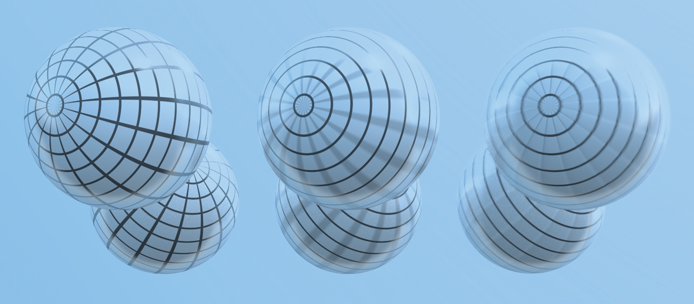
Figure 1: simulating the effect of movement using keyframe transformations
To achieve this effect, we will allow our renderer to support the specification of keyframe transformations, which are associated with a point in time. This makes it possible for the camera to move and for objects in the scene to be moving during the time the simulated camera’s shutter is open. The renderer will achieve this effect by interpolating between the keyframe matrices.
In order to interpolate between transform matricies, we can use an approach called matrix decomposition. Given a transformation matrix \(M\), we decompose it into a concatenation of scale (\(S\)), rotation (\(R\)) and translation (\(T\)) transformations:
\[ M = SRT \]
While interpolation between translation and scale matricies can be performed easily using linear interpolation, interpolating rotations is more difficult. To understand them, we will first dive into an alternative method of representing rotations: quaternions. Using quaternions provides an effective method of interpolating between rotations.
1.7.1 Quaternions
Quaternions are a four-dimensional number system. Just as the complex numbers can be considered to be a two-dimensional extension of the real numbers, quaternions are a four-dimensional extension of the complex numbers. Their properties make them particularly convenient for representing rotation in three dimensions.
Complex numbers and 2d rotation
To understand quaternions as a means of representing 3D rotation, it's useful to consider how the complex numbers can represent rotation in 2d space. A complex number consists of two values: a 'real' part, and an 'imaginary' part, where the imaginary part is some coefficient of the constant \(i = \sqrt{-1}\). Here are some examples:
\[ 3 + 5i \\ 1 + 2i \\ 6 + 4i \\ \]
To multiply two complex numbers, we multiply each term in the first number by each term in the second number. In places where we encounter \(i^2\), we can substitute with -1, as we know that \(i = \sqrt{-1}\). For example:
\[ (1 + 4i)(5 + i)\\ = (1)(5) + (1)(i) + (4i)(5) + (4i)(i)\\ = 5 + i + 20i + 4i^2\\ = 5 + 21i + 4i^2\\ = 5 + 21i + 4(-1)\\ = 5 + 21i - 4\\ = 1 + 21i\\ \]
We can imagine the complex numbers as existing on a 2D plane, where the real component represents the (x) axis, ad the (y) component represents the imaginary axis.
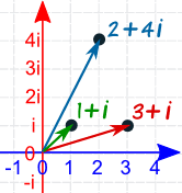
Figure 2: Complex numbers represented in a 2D plane.
This means that we can think of complex numbers as 2D vectors -- for example, the complex number \(2 + 4i\) above is the same as the 2D vector \((2, 4)\). This relationship has some useful properties. For example, we can rotate a vector by an angle \(\theta\) by converting it to a complex number and multiplying it by another complex number \(c = \cos(\theta) + i \sin(\theta)\). We can also multiply one vector by another to rotate the first vector by the angle of the second.
For example, in Figure 3, we have three vectors: red: \((1, 1)\), green: \((0, 1)\), and blue: \((-1, 1)\).
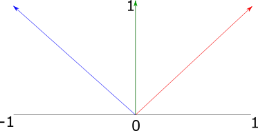
Figure 3: Three two-dimensional unit vectors, where the blue vector has an angle equal to the sum of the angles of the red and green vectors
The red vector has an angle of \(45^\circ\), and the green vector has an angle of \(90^\circ\). We can convert them to complex numbers and multiply them as follows:
\[ (red)(green) = \\ (1 + 1i)(0 + 1i) = \\ (1)(0) + 1i + (1i)(0) + (1i)(1i) = \\ 1i + 1i^2 = \\ 1i + -1 = \\ -1 + 1i = \\ (-1, 1) \]
The result \(-1, 1\) is equal to the blue vector in Figure 3, which has an angle of \(135^\circ\). Multiplying the complex numbers also results in the scaling of the magnitudes (not shown in this example, as we dealt with unit vectors). It turns out that the algebraic properties of complex numbers all have intuitive geometric interpretations -- multiplication applies scaling and rotation as demonstrated here; dividing has the opposite effect, and addition and subtraction work in the same way as vector addition and subtraction.
One might think that, to extend this pattern into three dimensions, we could come up with a new kind of complex number with two imaginary parts \(i\) and \(j\), where both \(i\) and \(j\) = \(\sqrt{-1}\). However, it turns out that this kind of 'triple' does not have the properties we need from a number system. For example, there is no way of defining multiplication and division on these triples such that division is the inverse of multiplication. However, it is possible to create a number system with the desired properties by extending the complex numbers into four dimensions.
Quaternions
Quaternions are four-dimensional numbers with the following form:
\[ q = (x, y, z, w) \\ = w + xi + yj + zk \]
\(i\), \(j\) and \(k\) are defined such that \(i^2 = j^2 = k^2 = ijk = -1\). We can also represent quaternions as \((q_{xyz}, q_w)\), where \(q_{xyz}\) is the imaginary 3-vector and \(q_w\) is the real part. Multiplication of two quaternions can be expressed in terms of the dot and cross products:
\[ (qq')_{xyz} = q_{xyz} \times q_{xyz} + q_wq'_{xyz} + q'_wq_{xyz} \\ (qq')_q = q_wq'_w - (q_{xyz} \cdot q'_{xyz}) \]
For the unit quaternions (that is, quaternions where the sum of squared components is 1), a 3D rotation of \(2\theta\) can be mapped to a quaternion \((\hat{v}, sin(\theta), cos(\theta)\)). We can then apply this to a point \(p\) represented in homogeneous coordinates with the following equation:
\[ p' = qpq^{-1} \]
To implement quaternions in rust, we can represent the imaginary part of the quaternion as a vector, and the real part as a scalar as follows:
#![allow(unused)]
fn main() {
struct Quaternion<T> {
    v: Vector3d,
    w: T
}
}
Arithmetic methods are implemented in a similar fashion to the Vector*, Point* and Normal3d types, in call cases simply using element-wise operations:
#![allow(unused)]
fn main() {
impl<T:Scalar> Add for Quaternion<T> {
    type Output = Quaternion<T>;
    fn add(self, other: Quaternion<T>) -> Quaternion<T> {
        Quaternion {
            v: self.v + other.v,
            w: self.w + other.w,
        }
    }
}
impl<T: Scalar> Sub for Quaternion<T> {
    type Output = Quaternion<T>;
    fn sub(self, other: Quaternion<T>) -> Quaternion<T> {
        Quaternion {
            v: self.v - other.v,
            w: self.w - other.w,
        }
    }
}
impl<T: Scalar> Mul<T> for Quaternion<T> {
    type Output = Quaternion<T>;
    fn mul(self, other: T) -> Quaternion<T> {
        Quaternion {
            v: self.v * other,
            w: self.w * other,
        }
    }
}
impl<T: Scalar> Div<T> for Quaternion<T> {
    type Output = Quaternion<T>;
    fn div(self, other: T) -> Quaternion<T> {
        Quaternion {
            v: self.v / other,
            w: self.w / other,
        }
    }
}
}
We additionally provide a dot() method for the inner product, and a normalize() method:
#![allow(unused)]
fn main() {
impl<T: Scalar + Float > Quaternion<T> {
    pub fn new(v: Vector3d<T>, w: T) -> Self {
        Quaternion{v, w}
    }
    pub fn dot(&self, other: &Self) -> T {
        self.v.dot(&other.v) + self.w * other.w
    }
    pub fn normalize(&self) -> Self {
        let norm = Scalar::sqrt(self.dot(&self));
        Quaternion{v: self.v / norm, w: self.w / norm}
    }
    ...
}
}
It is additionally useful to be able to convert a quaternion to and from a transformation matrix. The equation \(p' = qpq^{-1}\) for the quaternion product can be expanded to produce the following matrix which represents the same transformation:
\[ R(Q) = \begin{bmatrix} 2(q_0^2 + q_1^2) - 1 & 2(q_1q_2 - q_0q_3) & 2(q_1q_3 - q_0q_2) \\ 2(q_1q_2 - q_0q_3) & 2(q_0^2 + q_2^2) & 2(q_2q_3 - q_0q_1) \\ 2(q_1q_3 - q_0q_2) & 2(q_2q_3 - q_0q_1) & 2(q_0^2 + q_2^3) \\ \end{bmatrix} \]
This conversion and the conversion from matrix to quaternion are implemented in the from_transform() and to_transform() methods respectively.
Quaternion interpolation
The slerp() method interpolates between two quaternions using spherical linear interpolation. We can imagine this method as finding intermediate vectors along the surface of a sphere. This method has two desirable properties:
- Torque minimization, which means that it finds the shortest possible path between two rotations.
- Constant angular velocity, which means the relationship bewteen the interpolation parameter \(t\) and the change in rotation is constant.
Figure 4 visualizes the spherical linear interpolation problem. Our aim is to find an intermediate rotation \(q(t\) from \(q_0\) and \(q_1\) given the interpolation term \(t\). To simplify our understanding, we can imagine the rotation as taking place on a single 'slice' of the sphere, a unit circle.
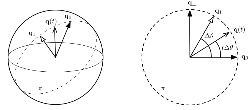
To solve the problem, we find a quaternion orthogonal to \(q_0\), \(q_\bot\). Then we just need to find the base and height of the triangle formed between \(q_1\) and \(q_0\) -- this is given by \(q(t) = q_0 \cos\theta' + q_1 \sin\theta'\).
To find \(q_\bot\), we project \(q_1\) on to \(q_0\) then subtract the orthogonal projection from q1. This is exactly the same pattern we used in the transformations section, when rotating a vector around an arbitrary axis:
\[ q_{\bot} = q_1 - (q_1 \cdot q_0) q_0 \]
Intermediate quaternions can now be found with:
\[ q(t) = q_0 \cos(\theta t) + \hat{q_{\bot}} \sin(\theta t) \]
Following the c++ pbrt implementation, the Slerp() function checks to see if the two quaternions are nearly parallel, in which case it uses regular linear interpolation of quaternion components in order to avoid numerical instability. Otherwise, it computes an orthogonal quaternion qperp and interpolation using the equations above.
#![allow(unused)]
fn main() {
impl<T: Scalar + Float > Quaternion<T> {
    ...
    pub fn slerp(&self, other: &Self, t: T) -> Self {
        let cos_theta = self.dot(other);
        if cos_theta  > T::one() - Scalar::epsilon() {
            return (*self * (T::one() - t) + *other * t).normalize();
        } else {
            let theta = clamp(cos_theta, -T::one(), T::one()).acos();
            let theta_p = theta * t;
            let qperp = (*other - *self * cos_theta).normalize();
            return *self * theta_p.cos() + qperp * theta_p.sin();
        }
    }
}
AnimatedTransform Implementation
Keyframe animation is implemented using the AnimatedTransform class. This class is constructed from two Transform instances which describe the start and end points of the animation, and a start_time and end_time which describe the time range of the movement. The struct definition looks like this:
#![allow(unused)]
fn main() {
pub struct AnimatedTransform<T> {
    start_transform: Transform<T>,
    end_transform: Transform<T>,
    start_time: T,
    end_time: T,
    translations: [Vector3d<T>; 2],
    scales: [Matrix4x4<T>; 2],
    rotations: [Quaternion<T>; 2],
}
}
The translations, scales and rotations arrays hold the decomposition of the start and endpoints into their component transforms. This is achieved through a decompose() method which is invoked from the AnimatedTransform constructor.
The decompose() method decomposes a transformation into its rotation, scaling, and translation components. It is not possible to know the exact transformations which actually generated a given composite transformation -- for example, given the matrix for the product of a translation and then a scale, an equal matrix could also be computed by first scaling and then translating (by different amounts). So instead, we treat all transformations as being composed of the same sequence:
\[ M = TRS \]
Where \(M\) is the transformation, \(T\) is a translation, \(R\) is a rotation, and \(S\) is scaling.
To find the translation \(T\), we just take the right-hand column of the input matrix:
\[ \begin{bmatrix} 1 & 0 & 0 & M_{03} \\ 0 & 1 & 0 & M_{13} \\ 0 & 0 & 1 & M_{23} \\ 0 & 0 & 0 & 1 \\ \end{bmatrix} \]
If we remove the translation component from the input matrix, we get a 3x3 matrix representing the scaling and rotation. To decompose this into the scaling and rotation matrices, we use a technique called polar decomposition. First, we extract the scaling matrix \(S\) by iteratively averating \(M\) with its inverse transpose until convergence. So we repeat this equation:
\[ M_i + 1 = \frac{1}{2}(M_i + (M^T_i)^{-1} ) \]
until the difference between \(M_i\) and \(M_{i+1}\) is a very small value.
Once we have the scaling matrix \(S\), we need to find \(R\) where \(SR = M\). We can get this by applying the matrix inverse as follows:
\[ R = S^{-1}M \]
In code, the decompose() method looks like this:
#![allow(unused)]
fn main() {
impl<T: Scalar + Float> AnimatedTransform<T> {
    ...
    pub fn decompose(matrix: Matrix4x4<T>) -> (Vector3d<T>, Quaternion<T>, Matrix4x4<T>){
        // Extract translation
        let translation = Vector3d::new(
            matrix.data[0][3],
            matrix.data[1][3],
            matrix.data[2][3]
        );
        // Compute rotation
        let mut rotation = Matrix4x4::default();
        let mut norm;
        let mut count = 0;
        loop {
            count+=1;
            let mut next = Matrix4x4::default();
            // Compute average of matrix and its inverse transpose
            let r_inverse_transpose = matrix.inverse().transpose();
            for i in 0..3 {
                for j in 0..3 {
                    next.data[i][j] = (matrix.data[i][j] + r_inverse_transpose.data[j][i]) * (T::two() / T::one());
                }
            }
            // Compute norm of difference -- when this is small enough, we're done
            norm = T::zero();
            for i in 0..3 {
                let n  = (matrix.data[i][0] - next.data[i][0]).abs() +
                (matrix.data[i][1] - matrix.data[i][1]).abs() +
                (matrix.data[i][2] - matrix.data[i][2]).abs();
                norm = Scalar::max(norm, n);
            }
            rotation = next;
            if norm < Scalar::epsilon() || count > 100 {
                break;
            }
        }
        // At this point, next contains the scale and rotation part of the matrix
        // To compute the scale, we need to find the matrix that satisfies
        // the equation M = RS. To get this, we just multiply M with the
        // inverse of R
        let scale = matrix * matrix.inverse().transpose();
        let rotation_qat = Quaternion::from_transform(&Transform::new(rotation, rotation.transpose()));
        return (translation, rotation_qat, scale);
    }
}
}
The decompose() method is invoked in the AnimatedTransform constructor, once for the start_transform and once for the end_transform. The results are stored on the AnimatedTransform instance to be used in the interpolate() method.
To perform the interpolation, we interpolate between each of the translation, scaling and rotation components, then multiply them together.
To interpolate a translation, we can interpolate linearly between the two vectors, using this formula:
\[ interpolated(V_1, V_2, t) = V_1(1 - t) + V_2t \]
This is similar to the linear interpolation formula introduced in the chapter on points -- one way to think about it is that we are treating the interpolation parameter \(t\) as a weight, which should give us \(V_2\) when the value is 1, some 'mix' of \(V_1\) and \(V_2\) when it is an intermediate value, and \(V_1\) when the value is 0.
To interpolate a scaling matrix, we can similarly interpolate linearly between the elements of the matrix:
\[ interpolated(A, B, t) = \\ \begin{bmatrix} A_{00}(1 - t) + B_{00}t&A_{01}(1 - t) + B_{01}t&A_{02}(1 - t) + B_{02}t&A_{03}(1 - t) + B_{03}t\\ A_{10}(1 - t) + B_{10}t&A_{11}(1 - t) + B_{11}t&A_{12}(1 - t) + B_{12}t&A_{03}(1 - t) + B_{13}t\\ A_{20}(1 - t) + B_{20}t&A_{21}(1 - t) + B_{21}t&A_{22}(1 - t) + B_{22}t&A_{03}(1 - t) + B_{23}t\\ A_{30}(1 - t) + B_{30}t&A_{31}(1 - t) + B_{31}t&A_{32}(1 - t) + B_{32}t&A_{03}(1 - t) + B_{33}t\\ \end{bmatrix} \]
To interpolate between the rotation quaterions, we use the Slerp procedure described in the chapter on Quaternions.
The final code for interpolating between transformations is shown below. It includes additional handling for boundary conditions -- if the interpolation parameter is outside the range of this AnimatedTransform, the value for the closest endpoint will be returned. Additionally, if the AnimatedTransform has the same start and end transformations, the starting point will be returned.
#![allow(unused)]
fn main() {
impl<T: Scalar + Float> AnimatedTransform<T> {
    ...
    pub fn interpolate(&self, time: T) -> Transform<T> {
        if !self.actually_animated {
            return self.start_transform.clone();
        }
        let mut t = (time - self.start_time) / (self.end_time - self.start_time);
        if t < T::zero() {
            t = T::zero();
        }
        if t > T::one() {
            t = T::one();
        }
        let translation = Transform::translate(self.translations[0] * (T::one() - t) + self.translations[1] * t);
        let scale = self.scales[0] * (T::one() - t) + self.scales[1] * t;
        let rotation = self.rotations[0].slerp(&self.rotations[1], t);
        let interpolated = &(&translation * rotation.to_transform()) * Transform::new(scale, scale.inverse());
        return interpolated;
    }
}
}
Geometry and Transformations
1.8 Interactions
Our ray tracer needs a way to represent information about points on 2D surfaces, which it will use in shading calculations.
In pbrt, this is achieved with the Interaction class, which defines the common data and methods for different kinds of interactions. Rust does not have a means for describing shared data for polymorphic types, so to achieve this, we provide two traits -- one with getters for the shared data elements, and one describing the shared methods.
#![allow(unused)]
fn main() {
pub trait InteractionData<T: Scalar> {
    //Location of this interaction
    fn point(&self) -> Point3d<T>;
    //Time of the interaction
    fn time(&self) -> T;
    //Floating point error
    fn p_error(&self) -> Vector3d<T>;
    //Negative direction of ray intersection
    fn wo(&self) -> Vector3d<T>;
    //Surface normal at this point, if this is an interaction with a surface
    fn n(&self) -> Option<Normal3d<T>> {
        None
    }
    //Flag representing whether or not this is a surface interaction
    fn is_surface_interaction(&self) -> bool {
        return self.n().is_some();
    }
    //Scattering medium at this point, if any
    fn medium_interface(&self) -> Option<&dyn MediumInterface>;
}
}
The InteractionMethods trait defines several methods for spawning rays as follows:
#![allow(unused)]
fn main() {
pub trait InteractionMethods<T: Scalar>: InteractionData<T> {
    fn spawn_ray(&self, direction: Vector3d<T>) -> Ray<T> {
        Ray::new(self.point(), direction, T::inf(), self.time())
    }
    fn spawn_ray_to_point(&self, point: Point3d<T>) -> Ray<T> {
        Ray::new(self.point(), point - self.point(), T::inf(), self.time())
    }
    fn spawn_ray_to_interaction(&self, other: &dyn InteractionMethods<T>) -> Ray<T> {
        Ray::new(self.point(), other.point() - self.point(), T::inf(), self.time())
    }
}
}
1.8.1 Surface Interactions
The geometry of a particular point on a surface (often a position found by intersecting a ray against the surface) is represented by a SurfaceInteraction. Having this abstraction lets most of the system work with points on surfaces without needing to consider the particular type of geometric shape the points lie on; the SurfaceInteraction abstraction supplies enough information about the surface point to allow the shading and geometric operations in the rest of pbrt to be implemented generically.
The SurfaceInteraction struct is defined as follows:
#![allow(unused)]
fn main() {
struct SurfaceInteraction<T: Scalar> {
    pub point: Point3d<T>,
    pub time: T,
    pub p_error: Vector3d<T>,
    pub wo: Vector3d<T>,
    pub n: Normal3d<T>,
    pub uv: Vector2d<T>,
    pub dp_du: Vector3d<T>,
    pub dp_dv: Vector3d<T>,
    pub dn_du: Normal3d<T>,
    pub dn_dv: Normal3d<T>,
    pub shading: Shading<T>,
    pub shape: Option<Box<dyn Shape<T>>>,
}
}
The first five fields correspond to those referred to in the InteractionData trait; getters are defined for these as part of the InteractionData impl block for SurfaceInteraction. The struct additionally stores uv, a 2d vector which provides a parameterized representation of the surface. The vectors dp_du and dp_dv represent the partial derivatives of the surface: \(\partial{p}/\partial{u}\) and \(\partial{p}/\partial{v}\). This allows us to represent the curvature of the surface.

Figure 1: Local Differential Geometry around a point \(p\)
The cross product of these partial derivatives gives us the surface normal as we move along the surface.
The SurfaceInteraction struct also stores a reference to the Shape it takes place on. Additionally, stores a second instance of a surface normal and the various partial derivatives to represent possibly perturbed values of these quantities as can be generated by bump mapping or interpolated per-vertex normals with triangles. Some parts of the system use this shading geometry, while others need to work with the original quantities. This is represented in a separate trait, the Shading trait. The SurfaceInteraction has an instance of Shading which is initialized at creation time and can be updated via the set_shading_geometry method.
The SurfaceInteraction new() constructor takes all of the above parameters as input, and computes the normal using the partial derivatives. It additionally reverses the direction of the normal in one of two situations:
- If the
Shapethat the interaction takes place on has areverse_orientationflag set totrue - If the
Shape's transformation matrix has switched the handedness of the object coordinate system from pbrt’s default left-handed coordinate system to a right-handed one
If both of the above conditions is true, we need the effects to cancel each other out, so an XOR (^) condition is used.
#![allow(unused)]
fn main() {
impl<T: Scalar> SurfaceInteraction<T> {
    pub fn new(
        point: Point3d<T>,
        time: T,
        p_error: Vector3d<T>,
        wo: Vector3d<T>,
        uv: Vector2d<T>,
        dp_du: Vector3d<T>,
        dp_dv: Vector3d<T>,
        dn_du: Normal3d<T>,
        dn_dv: Normal3d<T>,
        shape: Option<Box<dyn Shape<T>>>,
    ) -> Self {
            // Compute surface normal using partial derivatives
            let n = Normal3d::from_vec(dp_du.cross(&dp_dv).normalized());
            // Invert the normal based on properties of the shape
            let adjusted_normal = if shape.is_some() {
                if (shape.as_ref().unwrap().transform_swaps_handedness())
                ^ (shape.as_ref().unwrap().reverse_orientation()) {
                    -n
                } else {
                    n
                }
            } else {
                n
            };
            SurfaceInteraction {
                point,
                time,
                p_error,
                wo,
                n: adjusted_normal,
                uv,
                dp_du,
                dp_dv,
                dn_du,
                dn_dv,
                shading: Shading {
                    n,
                    dp_du,
                    dp_dv,
                    dn_du,
                    dn_dv
                },
                shape
        }
    }
}
}
Finally, we need a way of applying a transform to a SurfaceInteraction. For the most part, members are either transformed directly or copied, as appropriate, but given the approach that pbrt uses for bounding floating-point error in computed intersection points, transforming the p and pError member variables requires special care. The fragment that handles this, is defined in a later section (TODO: update!), when floating-point rounding error is discussed.
#![allow(unused)]
fn main() {
impl<T: Scalar> Mul<SurfaceInteraction<T>> for Transform<T> {
    type Output = SurfaceInteraction<T>;
    fn mul(self, other: SurfaceInteraction<T>) -> Self::Output {
        SurfaceInteraction {
            point: &self * other.point,
            time: other.time,
            p_error: &self * other.p_error,
            wo: &self * other.wo,
            n: &self * other.n,
            uv: other.uv,
            dp_du: &self * other.dp_du,
            dp_dv: &self * other.dp_dv,
            dn_du: &self * other.dn_du,
            dn_dv: &self * other.dn_dv,
            shading: Shading {
                n: &self * other.shading.n,
                dp_du: &self * other.shading.dp_du,
                dp_dv: &self * other.shading.dp_dv,
                dn_du: &self * other.shading.dn_du,
                dn_dv: &self * other.shading.dn_dv
            },
            shape: other.shape
        }
    }
}
}
Shapes
This section describes the implementation of geometric primitives such as spheres and triangles. All geometric primitives implement a common interface, such that the rest of the renderer can use this interface without needing any details about the underlying shape. This makes it possible to separate the geometric and shading subsystems.
pbrt-rust follows the original c++ implementation in using a two-level abstraction to represent shapes. The Shape trait provides access to the raw geometric properties of the primitive, such as its surface area and bounding box; it also provides a ray intersection routine. The Primitive trait encapsuraltes additional non-geometric information about the primitive, such as material properties. The rest of the render then deals only with the Primitive methods.
This chapter will focus on the geometry-only Shape interface, with the Primitive interface addressed in the following chapter.